What is meant by inferential statistics? What is the difference of descriptive and inferential statistics?. The Complete Data Science Developer Course 2023 [Videos].

Inferential statistics use measurements from the sample of subjects in the experiment to compare the treatment groups and make generalizations about the larger population of subjects. There are many types of inferential statistics and each is appropriate for a specific research design and sample characteristics. Descriptive statistics summarize the characteristics of a data set. Inferential statistics allow you to test a hypothesis or assess whether your data is generalizable to the broader population.

In this Video, I am going to discuss Descriptive Statistics in Data Science. Please read our previous Video where we discussed  At the end of this Video, you will understand the following pointers in detail which are related to Descriptive Statistics in Data Science.

1. Central Tendency Measures
2. The Story of Average
3. Dispersion Measures
4. Data Distributions
5. Central limit theorem
6. Sampling
7. Sampling Methods

Central Tendency Measures

A summary statistic that represents the centre point or typical value of a dataset is referred to as a measure of central tendency. These measures, also known as the central location of distribution, indicate where the majority of values in a distribution fall. Consider it the tendency of data to cluster around a middle value. The mean, median, and mode are the three most common measures of central tendency in statistics. Each of these measures employs a different method to determine the location of the central point.

The three distributions below represent different data conditions. In each distribution, look for the region where the most common values fall. Even though the shapes and types of data are different, you can find that central location. That’s the area in the distribution where the most common values are located.

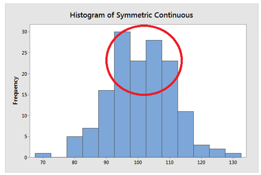
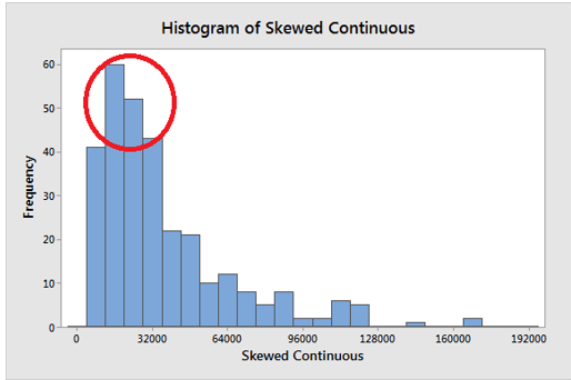
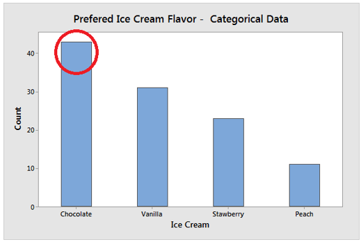
As the graphs show, you can see where the majority of the values occur. That is the idea. Measures of central tendency assign a numerical value to this concept. Coming up, you’ll discover that the best measure of central tendency changes as the distribution and type of data change. As a result, before selecting a measure of central tendency, you must first understand the type of data you have and graph it!

The central tendency of a distribution is one of the distribution’s characteristics. Another consideration is the variation around that central value. The graph below demonstrates how two distributions with the same central tendency (mean = 100) can be quite different. The distribution on the left is tightly clustered around the mean, whereas the distribution on the right is more spread out. It is critical to recognize that the central tendency only summarizes one aspect of distribution and thus provides an incomplete picture on its own.

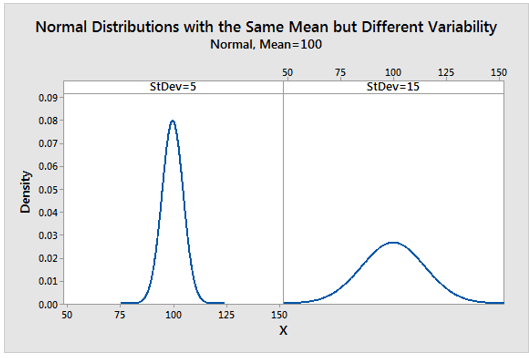
Mean Descriptive Statistics in Data Science

The mean is the arithmetic average, and it is probably the most familiar measure of central tendency. It is very simple to compute the mean. Simply add all of the values together and divide by the number of observations in your dataset.

The mean calculation takes into account all of the values in the data. The mean changes when any value is changed. The mean, on the other hand, does not always accurately locate the data’s centre. Look at the histograms below.

In a symmetric distribution, the mean locates the centre accurately.

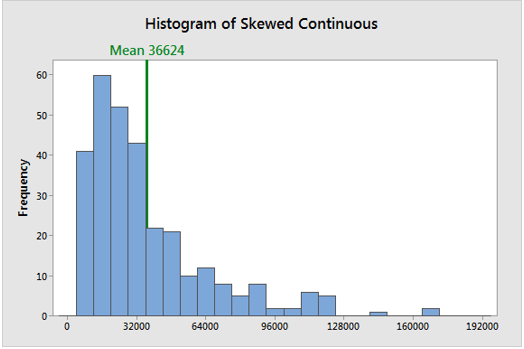
The mean, on the other hand, can be off in a skewed distribution. It is beginning to fall outside of the central area in the histogram above. This issue arises because outliers have a significant impact on the mean. The extreme values in a long tail pull the mean away from the centre. The mean moves away from the centre of the distribution as the distribution becomes more skewed. As a result, when dealing with a symmetric distribution, it is best to use the mean as a measure of central tendency.

Median Descriptive Statistics in Data Science

The median is the value in the middle. It’s the number that divides the dataset in half. To find the median, sort your data from smallest to largest, then look for the data point with an equal number of values above and below it. The method for determining the median differs slightly depending on whether your dataset has an even or odd number of values. I’ll show you how to calculate the median in both cases. For the sake of simplicity, I’ve used whole numbers in the examples below, but you can use decimal places as well.

Notice how the number 12 has six values above it and six values below it in the dataset with the odd number of observations. As a result, 12 is the dataset’s median.

When there is an even number of values, take the average of the two innermost values. The arithmetic mean of 27 and 29 is 28. As a result, the median of this dataset is 28.

Outliers and skewed data have less of an impact on the median. To understand why, consider the Median dataset below, where the median is 46. However, we discover data entry errors and must change four values in the Median Fixed dataset, which are shaded. We’ll raise them all significantly, resulting in a skewed distribution with large outliers.

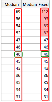
As you can see, the median remains constant. It’s still 46 degrees outside. The median value, unlike the mean, is not affected by all of the values in the dataset. As a result, when some of the values are more extreme, the effect on the median is less pronounced. Of course, the median can change as a result of other types of changes. When a distribution is skewed, the median is a better measure of central tendency than the mean.

The mode is the most frequently occurring value in your data set. The mode is the highest bar on a bar chart. A multimodal distribution exists when the data contains multiple values that are tied for the most frequent occurrence. If no value repeats, the data lacks a mode. The value 5 occurs the most frequently in the dataset below, making it the mode. These numbers could represent a 5-point Likert scale.

The mode is typically used with categorical, ordinal, and discrete data. In fact, the mode is the only measure of central tendency that can be applied to categorical data, such as the most popular ice cream flavour. However, because you can’t order the groups in categorical data, there isn’t a central value. The mode of ordinal and discrete data can be a value that is not in the centre. Once again, the mode denotes the most common value.

Dispersion Measures

The measures of central tendency are insufficient for describing data. Two data sets with the same mean can be completely different. To describe data, one must first understand the extent of variability. The measures of dispersion provide this information. The three most commonly used measures of dispersion are range, interquartile range, and standard deviation.

Range

The range is the difference between the data’s largest and smallest observations. The primary benefit of this measure of dispersion is that it is simple to compute. On the other hand, it has a slew of drawbacks. It is extremely sensitive to outliers and does not make use of all of the observations in a data set. Providing the minimum and maximum values rather than the range is more informative.

Interquartile Range

The difference between the 25th and 75th percentiles is defined as the interquartile range (also called the first and third quartile). As a result, the interquartile range describes the middle 50% of observations. If the interquartile range is large, it means that the middle 50% of observations are widely separated. The main advantage of the interquartile range is that it can be used as a measure of variability even if the extreme values are not recorded precisely (as in the case of open-ended class intervals in the frequency distribution). Another advantage is that it is unaffected by extreme values. The main disadvantage of using interquartile range as a measure of dispersion is that it is not easily manipulable mathematically.

Standard Deviation

The most commonly used measure of dispersion is the standard deviation (SD). It is a measure of data spread around the mean. SD is defined as the square root of the sum of the squared deviations from the mean divided by the number of observations.

SD is a very useful measure of dispersion because, if the observations are from a normal distribution, 68 percent of them fall between mean 1 SD. 95 percent of observations are within 2 standard deviations of the mean, and 99.7 percent are within 3 standard deviations of the mean.

Another advantage of SD is that, in addition to mean, it can be used to detect skewness. SD has the disadvantage of being an ineffective measure of dispersion for skewed data.

Data Distributions

A distribution is formed by a sample of data, and by far the most well-known distribution is the Gaussian distribution, also known as the Normal distribution.

The distribution provides a parameterized mathematical function that can be used to calculate the probability for any single observation in the sample space. This distribution, known as the probability density function, describes the grouping or density of the observations. We can also compute the probability that an observation will have a value equal to or less than a given value. A cumulative density function is a summary of these relationships between observations.

For example, we might be interested in human ages, with individual ages representing observations in the domain and ages 0 to 125 defining the sample space. The distribution is a mathematical function that describes the relationship between different height observations.

Density Functions

The density or density functions of distribution are frequently used to describe it. Density functions describe how the proportion of data or the likelihood of the proportion of observations changes across the distribution’s range. Probability density functions and cumulative density functions are the two types of density functions.

1. The Probability Density function computes the likelihood of observing a given value.
2. The Cumulative Density function computes the likelihood of an observation being equal to or less than a given value.

The likelihood of a given observation in a distribution can be calculated using a probability density function, or PDF. It can also be used to summarise the likelihood of observations across the sample space of the distribution. PDF plots depict the familiar shape of a distribution, such as a bell curve for the Gaussian distribution.

Gaussian Distribution

The Gaussian distribution, named after Carl Friedrich Gauss, is at the heart of much of statistics. Surprisingly, data from many fields of study can be described using a Gaussian distribution, so much so that the distribution is often referred to as the “normal” distribution due to its prevalence.

Two parameters can be used to describe a Gaussian distribution:

1. Mean: The expected value of the distribution is denoted by the Greek lowercase letter mu.
2. Variance: The spread of observations from the mean, denoted by the Greek lowercase letter sigma raised to the second power (because the units of the variable are squared).

The standard deviation is a normalised calculation of variance that is commonly used.

Standard deviation: The normalised spread of observations from the mean, denoted by the Greek lowercase letter sigma.

The norm SciPy module allows us to work with the Gaussian distribution. To generate a Gaussian probability density function with a given sample space, mean, and standard deviation, use the norm.pdf() function.

Chi-Squared distribution

The chi-squared distribution is represented by the Greek letter chi (X) raised to the second power (X2). The chi-squared distribution, like the Student’s t-distribution, is used in statistical methods on data drawn from a Gaussian distribution to quantify uncertainty. The chi-squared distribution, for example, is used in the chi-squared statistical tests for independence. The chi-squared distribution is, in fact, used to derive the Student’s t-distribution.

The degrees of freedom, denoted k, is the only parameter of the chi-squared distribution. The sum of k squared observations drawn from a Gaussian distribution is used to calculate an observation in a chi-squared distribution.

Where chi is a chi-squared distribution observation, x is a Gaussian distribution observation, and k is the number of x observations, which is also the number of degrees of freedom for the chi-squared distribution.

Although the distribution has a bell-like shape, the distribution is not symmetric.

Central Limit Theorem

According to the central limit theorem, if you have a population with a mean and a standard deviation and take sufficiently large random samples from the population with a replacement text annotation indicator, the distribution of the sample means will be approximately normally distributed. This is true regardless of whether the source population is normal or skewed, as long as the sample size is large enough (usually n > 30).

The theorem holds true even for samples smaller than 30 if the population is normal. This is true even if the population is binomial, as long as min(np, n(1-p))> 5, where n is the sample size and p is the probability of success in the population. This means that we can use the normal probability model to quantify uncertainty when inferring a population mean from a sample mean.

For the random samples we take from the population, we can compute the mean of the sample means:

Sampling Descriptive Statistics in Data Science

The selection of a subset (a statistical sample) of individuals from within a statistical population to estimate characteristics of the entire population is known as sampling. Statisticians strive to ensure that the samples accurately represent the population under consideration. Sampling has two advantages over measuring the entire population: lower cost and faster data collection.

Sampling Methods

1. Purely random sample

Each individual is chosen entirely by chance in this case, and each member of the population has an equal chance, or probability, of being chosen. One method for obtaining a random sample is to assign a number to each individual in a population and then use a table of random numbers to determine which individuals to include. 1 For example, if you have a sampling frame of 1000 individuals labelled 0 to 999, select your sample using groups of three digits from the random number table. So, if the first three numbers in the random number table were 094, choose the person labelled “94,” and so on.

2. Statistical sampling

Individuals are drawn at random from the sampling frame at regular intervals. The intervals are chosen to ensure that sufficient sample size is obtained. If you need a sample size n from a population of size x, you should take a sample from every x/nth individual. If you wanted a sample size of 100 from a population of 1000, for example, choose every 1000/100 = 10th member of the sampling frame.

Systematic sampling is frequently more convenient than simple random sampling, and it is simple to implement.

3. Stratified sample selection

The population is first divided into subgroups (or strata) that all share a similar characteristic in this method. It is used when we can reasonably expect the measurement of interest to differ between subgroups and we want to ensure that all subgroups are represented. In a study of stroke outcomes, for example, we might stratify the population by gender to ensure equal representation of men and women. The study sample is then created by randomly selecting equal sample sizes from each stratum. It may also be appropriate in stratified sampling to select non-equal sample sizes from each stratum.

4. Sampling by clusters

Individuals are not used as the sampling unit in a clustered sample, but rather subgroups of the population. The population is divided into subgroups known as clusters, which are chosen at random to participate in the study. Clusters are typically pre-defined; for example, individual GP practises or towns may be designated as clusters. All members of the selected clusters are then included in the study using single-stage cluster sampling. In two-stage cluster sampling, a random sample of individuals from each cluster is chosen for inclusion. Clustering should be considered in the analysis.